Why the NYC TLC trip record data is a nice training dataset for Data Engineers
·The New York City Taxi & Limousine Commission Trip Record Data is a really nice dataset to get started with Data Engineering or teaching it.
It has several nice properties that make it quite useful that we will show in this article.
We will look at this data using only pandas, not introducing any other tooling.
Many properties are nice for teaching different problems in Data Engineering.
Still, these properties are not so dominant that you would have to deal with all of them immediately but you can introduce concept-by-concept by using the data as an example problem.
In addition to this article, you can also access the content as a Jupyter Notebook. The notebook has the same content as the article but you can interactively reproduce the things mentioned here.
As a first step to better handle the data, we convert one of the files to Apache Parquet.
This enables us to get started much faster when loading the data a second time.
For a more in-depth reasoning on why to use Parquet, I’ve made a write-up on efficient DataFrame storage at one of my former employments.
The dataset comes as a collection of CSV files.
As such, CSV files come with no type information and types are then inferred by the reading library.
pandas does it best as detecting the correct ones but for some columns, we need to give it hints on what the correct ones are.
if not os.path.exists("yellow_tripdata_2016-01.parquet"):
    df = pd.read_csv(
        "../data/yellow_tripdata_2016-01.csv",
        dtype={"store_and_fwd_flag": "bool"},
        parse_dates=["tpep_pickup_datetime", "tpep_dropoff_datetime"],
        index_col=False,
        infer_datetime_format=True,
        true_values=["Y"],
        false_values=["N"],
    )
    df.to_parquet("yellow_tripdata_2016-01.parquet")
While a single month of the data still fits easily into the main memory of a laptop, the whole dataset is so large that you won’t be able to fit it into main memory of a consumer device. As you can see below, just the yellow cabs from 2009 until today need 225 GB of storage in CSV and the whole dataset using all available vehicle types add up to 267 GB.
This makes it very well suited to use it in exercises where you don’t want someone to be able to compute the result easily in main memory using just pandas but actually show the needs for additional tooling.
While the size is already a nice property, we can have a look at the data itself. For that, we load a single month into memory and have a brief look into it with pandas.
df = pd.read_parquet("yellow_tripdata_2016-01.parquet")
df.head()
#    VendorID tpep_pickup_datetime tpep_dropoff_datetime  passenger_count  trip_distance  pickup_longitude  ...  extra  mta_tax  tip_amount  tolls_amount  improvement_surcharge  total_amount
# 0         2           2016-01-01            2016-01-01                2           1.10        -73.990372  ...    0.5      0.5         0.0           0.0                    0.3           8.8
# 1         2           2016-01-01            2016-01-01                5           4.90        -73.980782  ...    0.5      0.5         0.0           0.0                    0.3          19.3
# 2         2           2016-01-01            2016-01-01                1          10.54        -73.984550  ...    0.5      0.5         0.0           0.0                    0.3          34.3
# 3         2           2016-01-01            2016-01-01                1           4.75        -73.993469  ...    0.0      0.5         0.0           0.0                    0.3          17.3
# 4         2           2016-01-01            2016-01-01                3           1.76        -73.960625  ...    0.0      0.5         0.0           0.0                    0.3           8.8
#
# [5 rows x 19 columns]
The first nice property one doesn’t realise anymore is that the data fits into a table and thus is well-suited for a pandas.DataFrame.
Other types of data, e.g. emails can surely be loaded into a DataFrame but is not as straight forward as the taxi data.
While we may want to also look at how to transform such data into tabular format, we slowly want to introduce people to it.
By using a dataset that is already tabular, we can gradually introduce new concepts instead of requiring them before we even have the data in pandas.
df.info()
# <class 'pandas.core.frame.DataFrame'>
# RangeIndex: 10906858 entries, 0 to 10906857
# Data columns (total 19 columns):
# VendorID                 int64
# tpep_pickup_datetime     datetime64[ns]
# tpep_dropoff_datetime    datetime64[ns]
# passenger_count          int64
# trip_distance            float64
# pickup_longitude         float64
# pickup_latitude          float64
# RatecodeID               int64
# store_and_fwd_flag       bool
# dropoff_longitude        float64
# dropoff_latitude         float64
# payment_type             int64
# fare_amount              float64
# extra                    float64
# mta_tax                  float64
# tip_amount               float64
# tolls_amount             float64
# improvement_surcharge    float64
# total_amount             float64
# dtypes: bool(1), datetime64[ns](2), float64(12), int64(4)
# memory usage: 1.5 GB
About half of all columns are floating point but we also have integers, booleans and even datetime types.
This gives us a wide range of types we can work on but still omits the types where the handling with Pandas isn’t as good as with those included.
For the types in the dataset, pandas and numpy provide highly optimised routines and we can use their plain-and-simple APIs to get decent performance.
This is really good to start with the basics and not need to dive into more low-level techniques to efficiently handle the data even though one has a datatype that is not supported by them.
Strings would be a typical datatype that will occur quite often in real-life datasets but currently pandas doesn’t have good native support for it.
It is represented as object datatype which basically means that all routines on it fall back to pure Python and cannot make use of the highly optimised numpy algorithms.
Looking at the different values a column has, we see that we have some high entropy columns, some medium entropy and some low entropy columns. This gives us a good mix of column values for aggregation operations.
# This takes quite some time to compute as the high entropy columns have expensive set operations.
df.nunique()

# VendorID                       2
# tpep_pickup_datetime     2368616
# tpep_dropoff_datetime    2372528
# passenger_count               10
# trip_distance               4513
# pickup_longitude           35075
# pickup_latitude            62184
# RatecodeID                     7
# store_and_fwd_flag             2
# dropoff_longitude          53813
# dropoff_latitude           87358
# payment_type                   5
# fare_amount                 1878
# extra                         35
# mta_tax                       16
# tip_amount                  3551
# tolls_amount                 940
# improvement_surcharge          7
# total_amount               11166
# dtype: int64
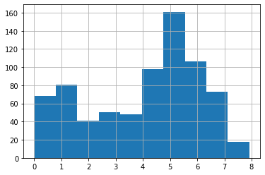
The data is even so dense that we can also use it to do simple streaming application tests. With on average 4 reqs/s, this doesn’t relate to real streaming applications but already gives a good start for the engineering challenges of such applications. And as the dataset is quite large, one can increase the pressure in streaming situations by supplying e.g. data for 10s in the actual time span of only 1s. This increases the load tenfold while still being able to test your streaming application for a year under this load.
events_per_minute = (
    df.iloc[:, 0]
    .groupby(
        by=[df["tpep_pickup_datetime"].dt.dayofyear, df["tpep_pickup_datetime"].dt.hour]
    )
    .count()
    / 60
    / 60
)

events_per_minute.min()
# 0.0022222222222222222
events_per_minute.mean()
# 4.072154271206691
events_per_minute.median()
# 4.694444444444445
events_per_minute.max()
# 7.919722222222222

events_per_minute.hist()
Machine Learning
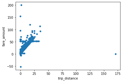
And finally, we can also use the data to do the most basic form of machine learning: linear regression. We can train a simple estimator that takes the trip distance and estimates the price.
df.sample(10000).plot.scatter(x="trip_distance", y="fare_amount")
As we only want to do a very basic estimation, we do a simple linear regression estimation.
cov_xy = (df["trip_distance"] * df["fare_amount"]).sum() - (
    df["trip_distance"].sum() * df["fare_amount"].sum()
) / len(df)
var_xy = (df["trip_distance"] ** 2).sum() - df["trip_distance"].sum() ** 2 / len(df)
beta = cov_xy / var_xy
alpha = df["fare_amount"].mean() - beta * df["trip_distance"].mean()

alpha
# 12.486907739140417
beta
# 4.6752084884145456e-06

# Select some sample data and see how well we can fit the price
sample = df.sample(10000)
sample["price"] = alpha + beta * sample["trip_distance"]
ax = sample.plot.scatter(x="trip_distance", y="fare_amount")
sample.plot.line(x="trip_distance", y="price", ax=ax, color="red")
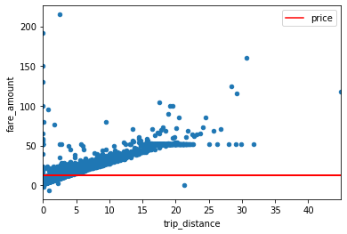
As one can see in the above image, as with any real life dataset, the New York City trip dataset also contains outliers that we need to clean to get a good regression. With the goal just showing the nice properties of the dataset, we aren’t doing any sophisticated cleaning here but simply get rid of the noisy data that disturbs our basic regression example.
cap_fare = df["fare_amount"].mean() + 3 * df["fare_amount"].std()
cap_distance = df["trip_distance"].mean() + 3 * df["trip_distance"].std()
df_filtered = df.query(
f"trip_distance > 0 and trip_distance < {cap_distance} and fare_amount > 0 and fare_amount < {cap_fare}"
)
# Train on the filtered data
cov_xy = (df_filtered["trip_distance"] * df_filtered["fare_amount"]).sum() - (
df_filtered["trip_distance"].sum() * df_filtered["fare_amount"].sum()
) / len(df_filtered)
var_xy = (df_filtered["trip_distance"] ** 2).sum() - df_filtered[
"trip_distance"
].sum() ** 2 / len(df_filtered)
beta = cov_xy / var_xy
alpha = df_filtered["fare_amount"].mean() - beta * df_filtered["trip_distance"].mean()
alpha
# 4.651606864471554
beta
# 2.661444816924383
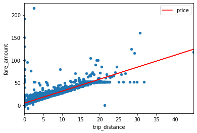
# Plot and check whether it fits better this time
sample["price"] = alpha + beta * sample["trip_distance"]
ax = sample.plot.scatter(x="trip_distance", y="fare_amount")
sample.plot.line(x="trip_distance", y="price", ax=ax, color="red")
Schema changes
Another thing that represents real life issues is that the dataset has a small schema change throughout its history. The columns used in 2015 and in 2018 aren’t exactly the same. The location columns have changed from providing coordinates for pickup and dropoff to using location IDs in later datasets
This is nice as you can use the dataset to explain schema migrations and write methods handling that. Still, the schema change is so small, that you can easily work around it when you aren’t interested in dealing with it explicitly.
# First line of yellow_tripdata_2018-08.csv
columns_2018 = "VendorID,tpep_pickup_datetime,tpep_dropoff_datetime,passenger_count,trip_distance,RatecodeID,store_and_fwd_flag,PULocationID,DOLocationID,payment_type,fare_amount,extra,mta_tax,tip_amount,tolls_amount,improvement_surcharge,total_amount"
columns_2018 = set(columns_2018.split(","))

# First line of yellow_tripdata_2015-08.csv
columns_2016 = "VendorID,tpep_pickup_datetime,tpep_dropoff_datetime,passenger_count,trip_distance,pickup_longitude,pickup_latitude,RatecodeID,store_and_fwd_flag,dropoff_longitude,dropoff_latitude,payment_type,fare_amount,extra,mta_tax,tip_amount,tolls_amount,improvement_surcharge,total_amount"
columns_2016 = set(columns_2016.split(","))

print(f"""Removed columns: {columns_2016 - columns_2018}
Added columns: {columns_2018 - columns_2016}""")

# Removed columns: {'dropoff_longitude', 'dropoff_latitude', 'pickup_longitude', 'pickup_latitude'}
# Added columns: {'PULocationID', 'DOLocationID'}
Conclusion
As one can see in the above examples, the New York City Taxi & Limousine Commission Trip Record Data covers a wide range of basic Data Engineering problems. The data comes as a collection of CSV files and such one first needs to load the data and ensure that the column types are all correct. Furthermore, the most prominent feature of the dataset is its sheer size with well over 200GB of raw data, it is one of the few openly available large datasets. The main property that makes it suitable as an entry dataset is that it already comes in a flat tabular form. That means you can start directly working on it instead of spending a lot of time first to reshape the dataset to your actual use case.
The data is also nice that it has simple (but not too simple) properties that allow you train a machine learning model on it while teaching some of the basic concepts. As it is a real life dataset, you get unclean data and need to filter that to get meaningful results. Additionally, it is a living dataset such that the columns are not the same throughout the whole history. The schema change is so small that you can ignore it in most use cases but still it is existent and thus usable for a small session on how to handle these changes in a data pipeline.